11 Model building
11.1 Specify models
The process of specifying our models is always as follows:
- Pick a
model type - set the
engine - Set the
mode: regression or classification
You can choose the model type and engine from this list.
11.1.1 Logistic regression
log_spec <- # your model specification
  logistic_reg() %>%  # model type
  set_engine(engine = "glm") %>%  # model engine
  set_mode("classification") # model mode

# Show your model specification
log_spec
#> Logistic Regression Model Specification (classification)
#>
#> Computational engine: glm11.1.2 Random forest
library(ranger)
rf_spec <-
rand_forest() %>%
set_engine("ranger", importance = "impurity") %>%
set_mode("classification")When we set the engine, we add importance = "impurity". This will provide variable importance scores for this model, which gives some insight into which predictors drive model performance.
11.1.4 K-nearest neighbor
knn_spec <-
nearest_neighbor(neighbors = 4) %>% # we can adjust the number of neighbors
set_engine("kknn") %>%
set_mode("classification") 11.1.5 Neural network
To use the neural network model, you will need to install the following packages: keras. You will also need the python keras library installed (see ?keras::install_keras()).
library(keras)
nnet_spec <-
mlp() %>%
set_mode("classification") %>%
set_engine("keras", verbose = 0) We set the engine-specific verbose argument to prevent logging the results.
11.2 Create workflows
To combine the data preparation recipe with the model building, we use the package workflows. A workflow is an object that can bundle together your pre-processing recipe, modeling, and even post-processing requests (like calculating the RMSE).
11.2.1 Logistic regression
Bundle recipe and model with workflows:
log_wflow <- # new workflow object
workflow() %>% # use workflow function
add_recipe(housing_rec) %>% # use the new recipe
add_model(log_spec) # add your model spec
# show object
log_wflow#> ══ Workflow ════════════════════════════════════════════════════════════════════
#> Preprocessor: Recipe
#> Model: logistic_reg()
#>
#> ── Preprocessor ────────────────────────────────────────────────────────────────
#> 7 Recipe Steps
#>
#> ● step_log()
#> ● step_naomit()
#> ● step_novel()
#> ● step_normalize()
#> ● step_dummy()
#> ● step_zv()
#> ● step_corr()
#>
#> ── Model ───────────────────────────────────────────────────────────────────────
#> Logistic Regression Model Specification (classification)
#>
#> Computational engine: glm11.2.2 Random forest
Bundle recipe and model:
rf_wflow <-
 workflow() %>%
 add_recipe(housing_rec) %>%
 add_model(rf_spec)
11.2.3 XGBoost
Bundle recipe and model:
xgb_wflow <-
 workflow() %>%
 add_recipe(housing_rec) %>%
add_model(xgb_spec)11.3 Evaluate models
Now we can use our validation set (cv_folds) to estimate the performance of our models using the fit_resamples() function to fit the models on each of the folds and store the results.
Note that fit_resamples() will fit our model to each resample and evaluate on the heldout set from each resample. The function is usually only used for computing performance metrics across some set of resamples to evaluate our models (like accuracy) - the models are not even stored. However, in our example we save the predictions in order to visualize the model fit and residuals with control_resamples(save_pred = TRUE).
Finally, we collect the performance metrics with collect_metrics() and pick the model that does best on the validation set.
11.3.1 Logistic regression
We use our workflow object to perform resampling. Furthermore, we use
metric_set()to choose some common classification performance metrics provided by the yardstick package. Visit yardsticks reference to see the complete list of all possible metrics.
Note that Cohen’s kappa coefficient (κ) is a similar measure to accuracy, but is normalized by the accuracy that would be expected by chance alone and is very useful when one or more classes have large frequency distributions. The higher the value, the better.
log_res <-
  log_wflow %>%
  fit_resamples(
    resamples = cv_folds,
    metrics = metric_set(
      recall, precision, f_meas,
      accuracy, kap,
      roc_auc, sens, spec),
    control = control_resamples(
      save_pred = TRUE)
    )
11.3.1.1 Model coefficients
The above described method to obtain log_res is fine if we are not interested in model coefficients. However, if we would like to extract the model coeffcients from fit_resamples, we need to proceed as follows:
# save model coefficients for a fitted model object from a workflow
get_model <- function(x) {
  pull_workflow_fit(x) %>%
    tidy()
}

# same as before with one exception
log_res_2 <-
  log_wflow %>%
  fit_resamples(
    resamples = cv_folds,
    metrics = metric_set(
      recall, precision, f_meas,
      accuracy, kap,
      roc_auc, sens, spec),
    control = control_resamples(
      save_pred = TRUE,
      extract = get_model) # use extract and our new function
    )

log_res_2
#> # Resampling results
#> # 5-fold cross-validation using stratification
#> # A tibble: 5 x 6
#> splits id .metrics .notes .extracts .predictions
#> <list> <chr> <list> <list> <list> <list>
#> 1 <split [12.4K/… Fold1 <tibble [8 ×… <tibble [0… <tibble [1 ×… <tibble [3,097 …
#> 2 <split [12.4K/… Fold2 <tibble [8 ×… <tibble [0… <tibble [1 ×… <tibble [3,097 …
#> 3 <split [12.4K/… Fold3 <tibble [8 ×… <tibble [0… <tibble [1 ×… <tibble [3,096 …
#> 4 <split [12.4K/… Fold4 <tibble [8 ×… <tibble [0… <tibble [1 ×… <tibble [3,095 …
#> 5 <split [12.4K/… Fold5 <tibble [8 ×… <tibble [0… <tibble [1 ×… <tibble [3,095 …Now there is a .extracts column with nested tibbles.
log_res_2$.extracts[[1]]#> # A tibble: 1 x 2
#> .extracts .config
#> <list> <chr>
#> 1 <tibble [8 × 5]> Preprocessor1_Model1To get the results use:
log_res_2$.extracts[[1]][[1]]#> [[1]]
#> # A tibble: 8 x 5
#> term estimate std.error statistic p.value
#> <chr> <dbl> <dbl> <dbl> <dbl>
#> 1 (Intercept) -2.02 0.0510 -39.6 0.
#> 2 median_income -1.91 0.0470 -40.6 0.
#> 3 rooms_per_household 0.252 0.0376 6.70 2.14e-11
#> 4 population_per_household 0.485 0.0297 16.3 7.36e-60
#> 5 ocean_proximity_INLAND 2.92 0.0729 40.0 0.
#> 6 ocean_proximity_ISLAND -11.4 160. -0.0714 9.43e- 1
#> # … with 2 more rowsAll of the results can be flattened and collected using:
all_coef <- map_dfr(log_res_2$.extracts, ~ .x[[1]][[1]])Show all of the resample coefficients for a single predictor:
filter(all_coef, term == "median_income")#> # A tibble: 5 x 5
#> term estimate std.error statistic p.value
#> <chr> <dbl> <dbl> <dbl> <dbl>
#> 1 median_income -1.91 0.0470 -40.6 0
#> 2 median_income -1.91 0.0469 -40.6 0
#> 3 median_income -1.89 0.0469 -40.4 0
#> 4 median_income -1.96 0.0480 -40.8 0
#> 5 median_income -1.90 0.0468 -40.5 011.3.1.2 Performance metrics
Show average performance over all folds:
log_res %>% collect_metrics(summarize = TRUE)#> # A tibble: 8 x 6
#> .metric .estimator mean n std_err .config
#> <chr> <chr> <dbl> <int> <dbl> <chr>
#> 1 accuracy binary 0.849 5 0.00283 Preprocessor1_Model1
#> 2 f_meas binary 0.883 5 0.00243 Preprocessor1_Model1
#> 3 kap binary 0.672 5 0.00569 Preprocessor1_Model1
#> 4 precision binary 0.871 5 0.000987 Preprocessor1_Model1
#> 5 recall binary 0.896 5 0.00430 Preprocessor1_Model1
#> 6 roc_auc binary 0.918 5 0.00117 Preprocessor1_Model1
#> # … with 2 more rowsShow performance for every single fold:
log_res %>% collect_metrics(summarize = FALSE)#> # A tibble: 40 x 5
#> id .metric .estimator .estimate .config
#> <chr> <chr> <chr> <dbl> <chr>
#> 1 Fold1 recall binary 0.886 Preprocessor1_Model1
#> 2 Fold1 precision binary 0.868 Preprocessor1_Model1
#> 3 Fold1 f_meas binary 0.877 Preprocessor1_Model1
#> 4 Fold1 accuracy binary 0.842 Preprocessor1_Model1
#> 5 Fold1 kap binary 0.658 Preprocessor1_Model1
#> 6 Fold1 sens binary 0.886 Preprocessor1_Model1
#> # … with 34 more rows11.3.1.3 Collect predictions
To obtain the actual model predictions, we use the function collect_predictions and save the result as log_pred:
log_pred <-
  log_res %>%
  collect_predictions()
11.3.1.4 Confusion matrix
Now we can use the predictions to create a confusion matrix with conf_mat():
log_pred %>%
  conf_mat(price_category, .pred_class)
#> Truth
#> Prediction above below
#> above 8788 1306
#> below 1025 4361Additionally, the confusion matrix can quickly be visualized in different formats using autoplot(). Type mosaic:
log_pred %>%
  conf_mat(price_category, .pred_class) %>%
  autoplot(type = "mosaic")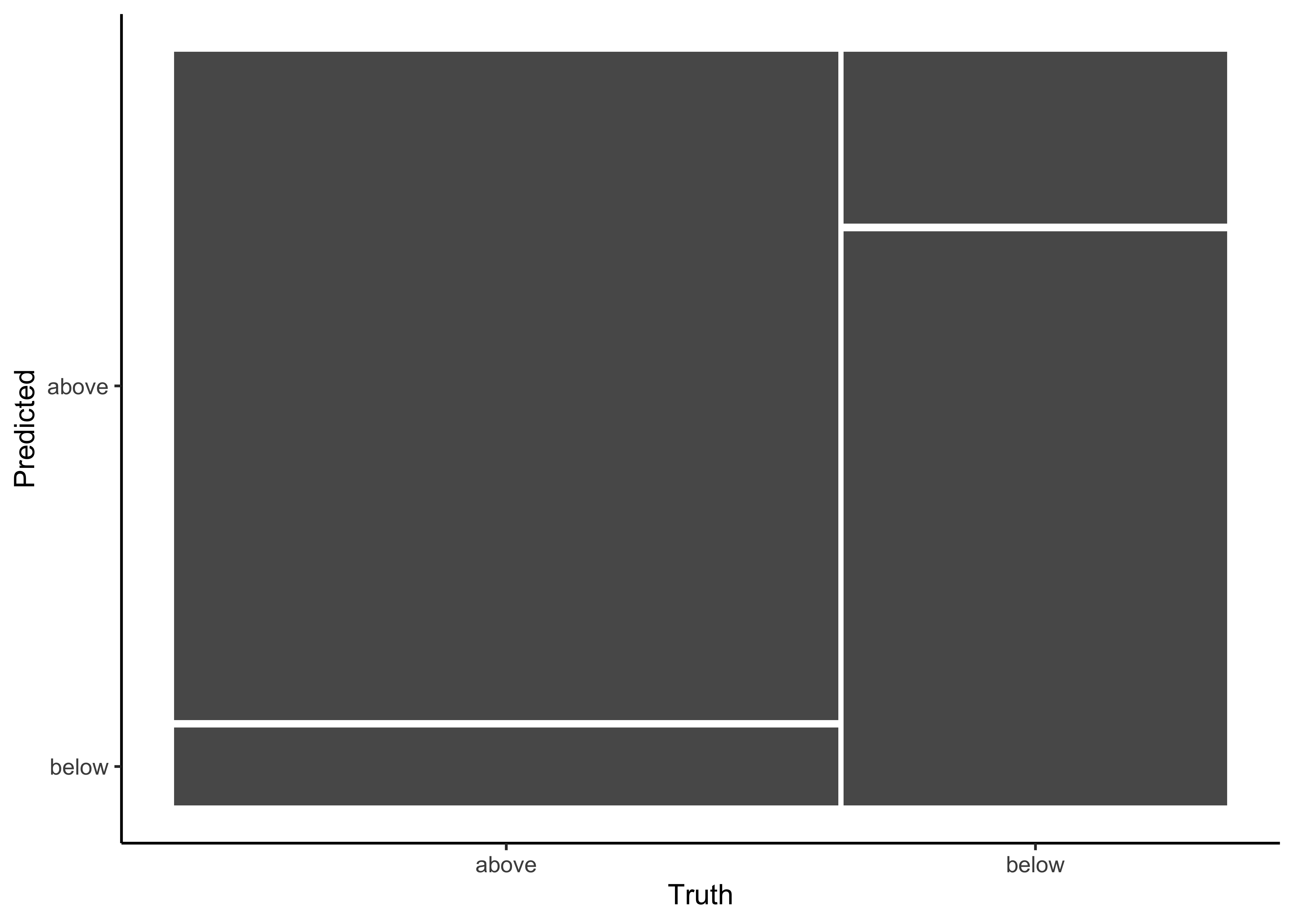
Or type heatmap:
log_pred %>%
  conf_mat(price_category, .pred_class) %>%
  autoplot(type = "heatmap")
11.3.1.5 ROC-Curve
We can also make an ROC curve for our 5 folds. Since the category we are predicting is the first level in the price_category factor (“above”), we provide roc_curve() with the relevant class probability .pred_above:
log_pred %>%
  group_by(id) %>% # id contains our folds
  roc_curve(price_category, .pred_above) %>%
  autoplot()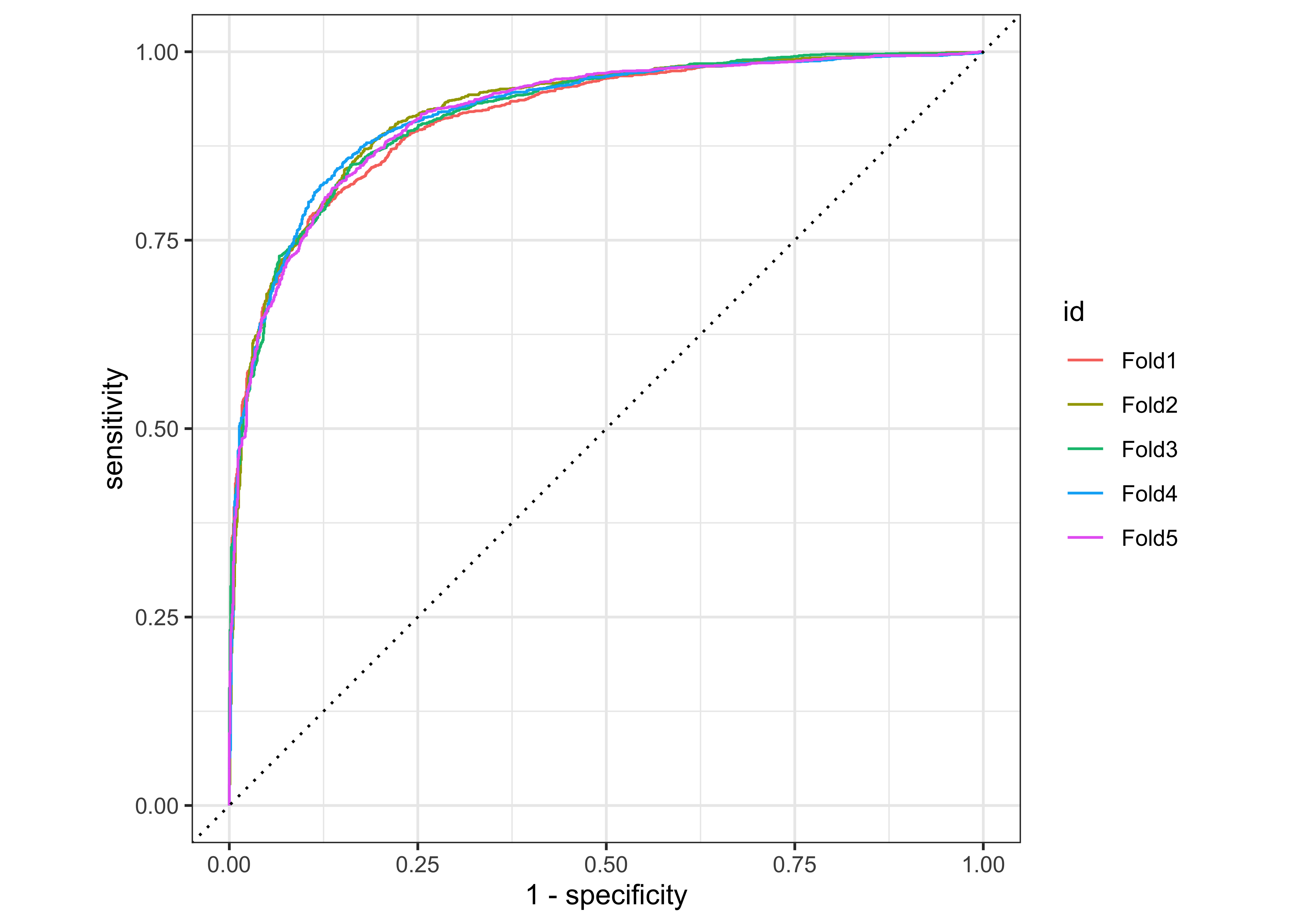
Visit Google developer’s Machine Learning Crashcourse to learn more about the ROC-Curve.
11.3.2 Random forest
We don’t repeat all of the steps shown in logistic regression and just focus on the performance metrics.
rf_res <-
  rf_wflow %>%
  fit_resamples(
    resamples = cv_folds,
    metrics = metric_set(
      recall, precision, f_meas,
      accuracy, kap,
      roc_auc, sens, spec),
    control = control_resamples(save_pred = TRUE)
    )

rf_res %>%  collect_metrics(summarize = TRUE)
#> # A tibble: 8 x 6
#> .metric .estimator mean n std_err .config
#> <chr> <chr> <dbl> <int> <dbl> <chr>
#> 1 accuracy binary 0.858 5 0.00316 Preprocessor1_Model1
#> 2 f_meas binary 0.889 5 0.00263 Preprocessor1_Model1
#> 3 kap binary 0.691 5 0.00656 Preprocessor1_Model1
#> 4 precision binary 0.877 5 0.00185 Preprocessor1_Model1
#> 5 recall binary 0.902 5 0.00435 Preprocessor1_Model1
#> 6 roc_auc binary 0.926 5 0.00187 Preprocessor1_Model1
#> # … with 2 more rows11.3.3 XGBoost
We don’t repeat all of the steps shown in logistic regression and just focus on the performance metrics.
xgb_res <-
  xgb_wflow %>%
  fit_resamples(
    resamples = cv_folds,
    metrics = metric_set(
      recall, precision, f_meas,
      accuracy, kap,
      roc_auc, sens, spec),
    control = control_resamples(save_pred = TRUE)
    )

xgb_res %>% collect_metrics(summarize = TRUE)
#> # A tibble: 8 x 6
#> .metric .estimator mean n std_err .config
#> <chr> <chr> <dbl> <int> <dbl> <chr>
#> 1 accuracy binary 0.859 5 0.00262 Preprocessor1_Model1
#> 2 f_meas binary 0.890 5 0.00235 Preprocessor1_Model1
#> 3 kap binary 0.694 5 0.00508 Preprocessor1_Model1
#> 4 precision binary 0.881 5 0.000480 Preprocessor1_Model1
#> 5 recall binary 0.898 5 0.00485 Preprocessor1_Model1
#> 6 roc_auc binary 0.928 5 0.00121 Preprocessor1_Model1
#> # … with 2 more rows11.3.4 K-nearest neighbor
We don’t repeat all of the steps shown in logistic regression and just focus on the performance metrics.
knn_res <-
  knn_wflow %>%
  fit_resamples(
    resamples = cv_folds,
    metrics = metric_set(
      recall, precision, f_meas,
      accuracy, kap,
      roc_auc, sens, spec),
    control = control_resamples(save_pred = TRUE)
    )

knn_res %>% collect_metrics(summarize = TRUE)
#> # A tibble: 8 x 6
#> .metric .estimator mean n std_err .config
#> <chr> <chr> <dbl> <int> <dbl> <chr>
#> 1 accuracy binary 0.803 5 0.00437 Preprocessor1_Model1
#> 2 f_meas binary 0.845 5 0.00361 Preprocessor1_Model1
#> 3 kap binary 0.575 5 0.00926 Preprocessor1_Model1
#> 4 precision binary 0.844 5 0.00402 Preprocessor1_Model1
#> 5 recall binary 0.846 5 0.00565 Preprocessor1_Model1
#> 6 roc_auc binary 0.883 5 0.00289 Preprocessor1_Model1
#> # … with 2 more rows11.3.5 Neural network
We don’t repeat all of the steps shown in logistic regression and just focus on the performance metrics.
nnet_res <-
  nnet_wflow %>%
  fit_resamples(
    resamples = cv_folds,
    metrics = metric_set(
      recall, precision, f_meas,
      accuracy, kap,
      roc_auc, sens, spec),
    control = control_resamples(save_pred = TRUE)
    )

nnet_res %>% collect_metrics(summarize = TRUE)
#> # A tibble: 8 x 6
#> .metric .estimator mean n std_err .config
#> <chr> <chr> <dbl> <int> <dbl> <chr>
#> 1 accuracy binary 0.857 5 0.00288 Preprocessor1_Model1
#> 2 f_meas binary 0.888 5 0.00244 Preprocessor1_Model1
#> 3 kap binary 0.689 5 0.00590 Preprocessor1_Model1
#> 4 precision binary 0.881 5 0.00173 Preprocessor1_Model1
#> 5 recall binary 0.895 5 0.00428 Preprocessor1_Model1
#> 6 roc_auc binary 0.927 5 0.00147 Preprocessor1_Model1
#> # … with 2 more rows11.3.6 Compare models
Extract metrics from our models to compare them:
log_metrics <-
  log_res %>%
  collect_metrics(summarise = TRUE) %>%
  mutate(model = "Logistic Regression") # add the name of the model to every row

rf_metrics <-
  rf_res %>%
  collect_metrics(summarise = TRUE) %>%
  mutate(model = "Random Forest")

xgb_metrics <-
  xgb_res %>%
  collect_metrics(summarise = TRUE) %>%
  mutate(model = "XGBoost")

knn_metrics <-
  knn_res %>%
  collect_metrics(summarise = TRUE) %>%
  mutate(model = "Knn")

nnet_metrics <-
  nnet_res %>%
  collect_metrics(summarise = TRUE) %>%
  mutate(model = "Neural Net")

# create dataframe with all models
model_compare <- bind_rows(log_metrics,
                           rf_metrics,
                           xgb_metrics,
                           knn_metrics,
                           nnet_metrics)

# change data structure
model_comp <-
  model_compare %>%
  select(model, .metric, mean, std_err) %>%
  pivot_wider(names_from = .metric, values_from = c(mean, std_err))

# show mean F1-Score for every model
model_comp %>%
  arrange(mean_f_meas) %>%
  mutate(model = fct_reorder(model, mean_f_meas)) %>% # order results
  ggplot(aes(model, mean_f_meas, fill=model)) +
  geom_col() +
  coord_flip() +
  scale_fill_brewer(palette = "Blues") +
   geom_text(
     size = 3,
     aes(label = round(mean_f_meas, 2), y = mean_f_meas + 0.08),
     vjust = 1
  )

# show mean area under the curve (auc) per model
model_comp %>%
  arrange(mean_roc_auc) %>%
  mutate(model = fct_reorder(model, mean_roc_auc)) %>%
  ggplot(aes(model, mean_roc_auc, fill=model)) +
  geom_col() +
  coord_flip() +
  scale_fill_brewer(palette = "Blues") +
     geom_text(
     size = 3,
     aes(label = round(mean_roc_auc, 2), y = mean_roc_auc + 0.08),
     vjust = 1
  )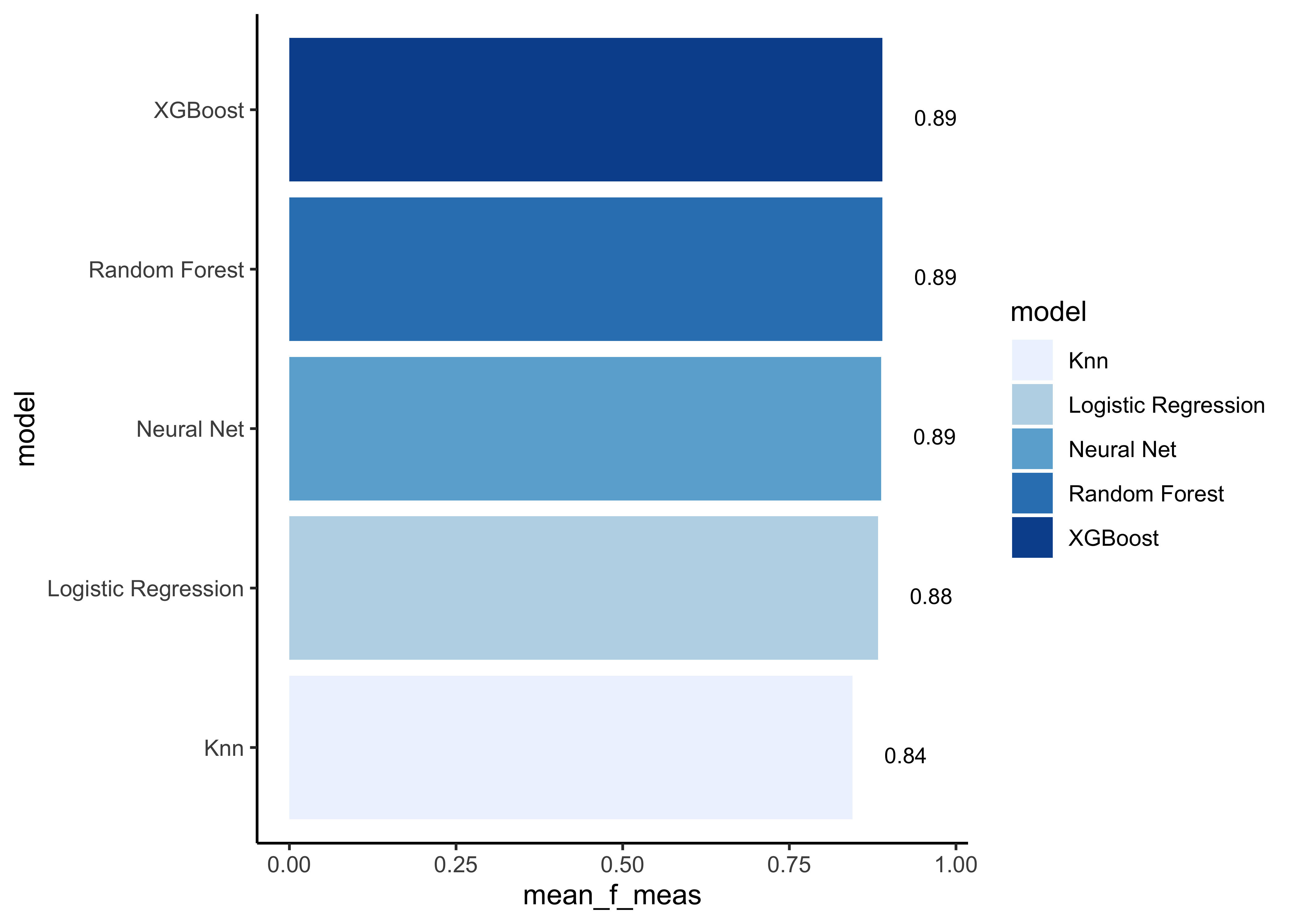

Note that the model results are all quite similar. In our example we choose the F1-Score as performance measure to select the best model. Let’s find the maximum mean F1-Score:
model_comp %>% slice_max(mean_f_meas)#> # A tibble: 1 x 17
#> model mean_accuracy mean_f_meas mean_kap mean_precision mean_recall
#> <chr> <dbl> <dbl> <dbl> <dbl> <dbl>
#> 1 XGBo… 0.859 0.890 0.694 0.881 0.898
#> # … with 11 more variables: mean_roc_auc <dbl>, mean_sens <dbl>,
#> # mean_spec <dbl>, std_err_accuracy <dbl>, std_err_f_meas <dbl>,
#> # std_err_kap <dbl>, std_err_precision <dbl>, std_err_recall <dbl>,
#> # std_err_roc_auc <dbl>, std_err_sens <dbl>, std_err_spec <dbl>Now it’s time to fit the best model one last time to the full training set and evaluate the resulting final model on the test set.
11.4 Last evaluation on test set
Tidymodels provides the function last_fit() which fits a model to the whole training data and evaluates it on the test set. We just need to provide the workflow object of the best model as well as the data split object (not the training data).
last_fit_rf <- last_fit(rf_wflow,
                        split = data_split,
                        metrics = metric_set(
                          recall, precision, f_meas,
                          accuracy, kap,
                          roc_auc, sens, spec)
                        )
Show performance metrics
last_fit_rf %>%
  collect_metrics()
#> # A tibble: 8 x 4
#> .metric .estimator .estimate .config
#> <chr> <chr> <dbl> <chr>
#> 1 recall binary 0.893 Preprocessor1_Model1
#> 2 precision binary 0.878 Preprocessor1_Model1
#> 3 f_meas binary 0.885 Preprocessor1_Model1
#> 4 accuracy binary 0.853 Preprocessor1_Model1
#> 5 kap binary 0.682 Preprocessor1_Model1
#> 6 sens binary 0.893 Preprocessor1_Model1
#> # … with 2 more rowsAnd these are our final performance metrics. Remember that if a model fit to the training dataset also fits the test dataset well, minimal overfitting has taken place. This seems to be also the case in our example.
To learn more about the model we can access the variable importance scores via the .workflow column. We first need to pluck out the first element in the workflow column, then pull out the fit from the workflow object. Finally, the vip package helps us visualize the variable importance scores for the top features. Note that we can’t create this type of plot for every model engine.
library(vip)

last_fit_rf %>%
  pluck(".workflow", 1) %>%
  pull_workflow_fit() %>%
  vip(num_features = 10)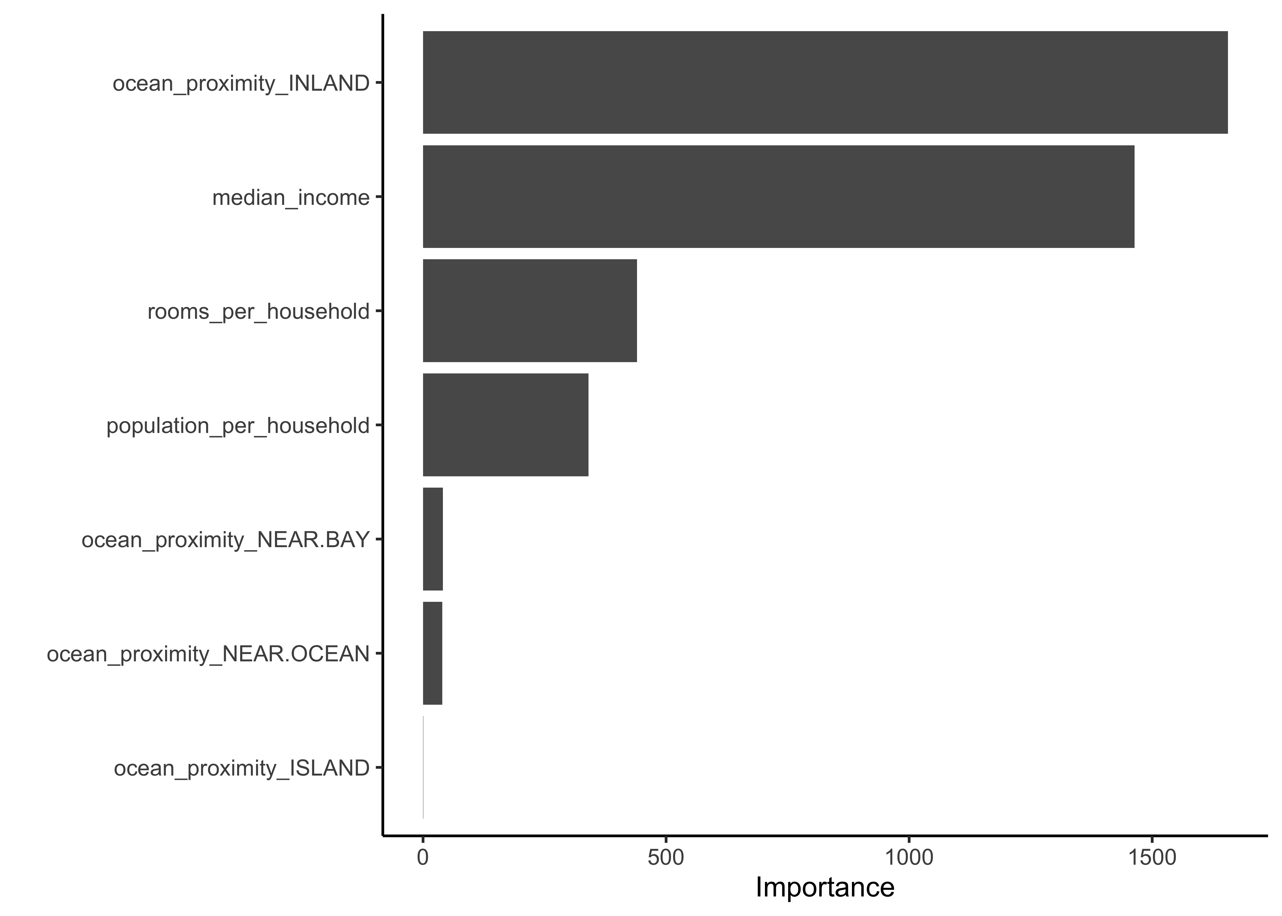
The two most important predictors in whether a district has a median house value above or below 150000 dollars were the ocean proximity inland and the median income.
Take a look at the confusion matrix:
last_fit_rf %>%
  collect_predictions() %>%
  conf_mat(price_category, .pred_class) %>%
  autoplot(type = "heatmap")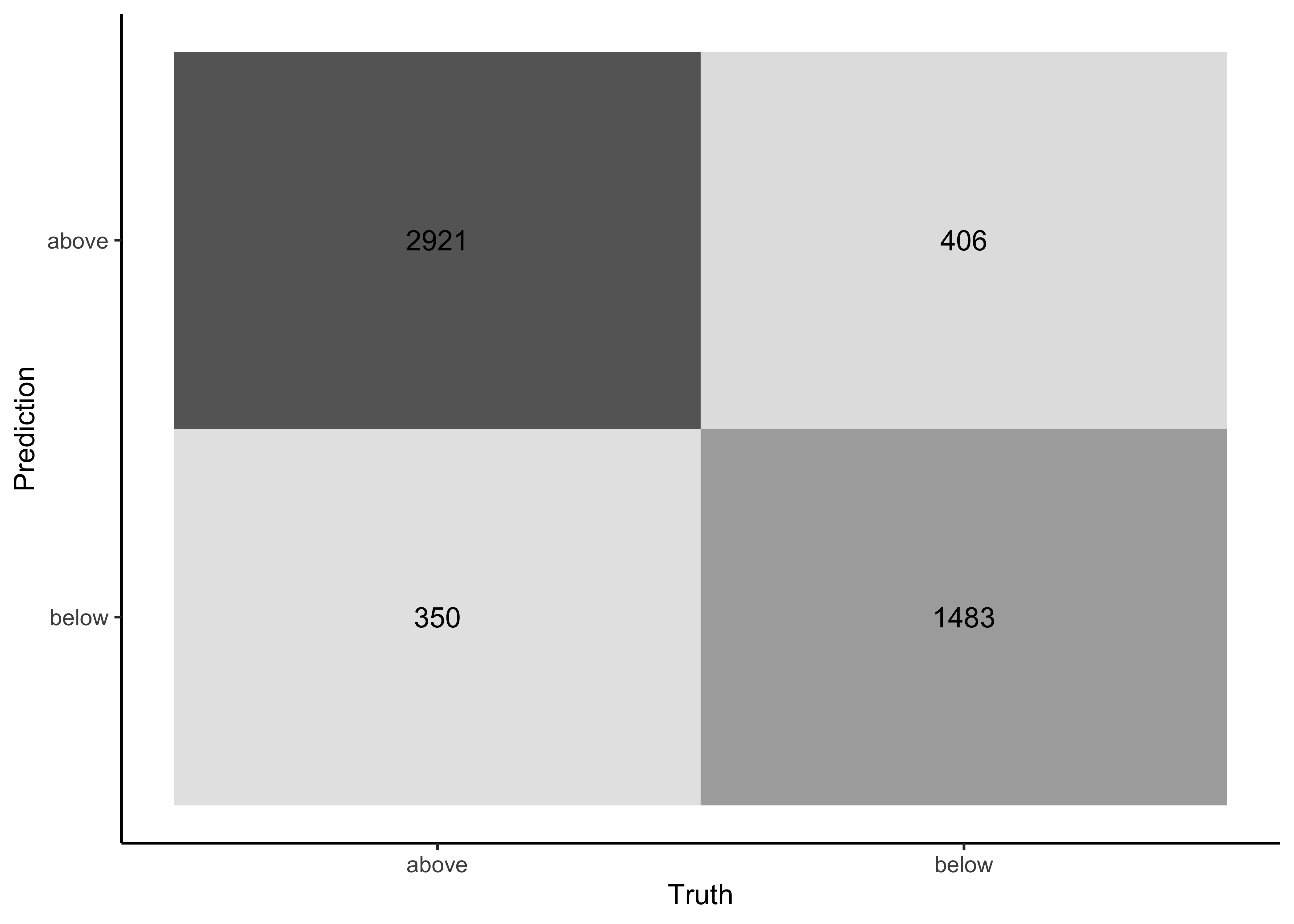
Let’s create the ROC curve. Again, since the event we are predicting is the first level in the price_category factor (“above”), we provide roc_curve() with the relevant class probability .pred_above:
last_fit_rf %>%
  collect_predictions() %>%
  roc_curve(price_category, .pred_above) %>%
  autoplot()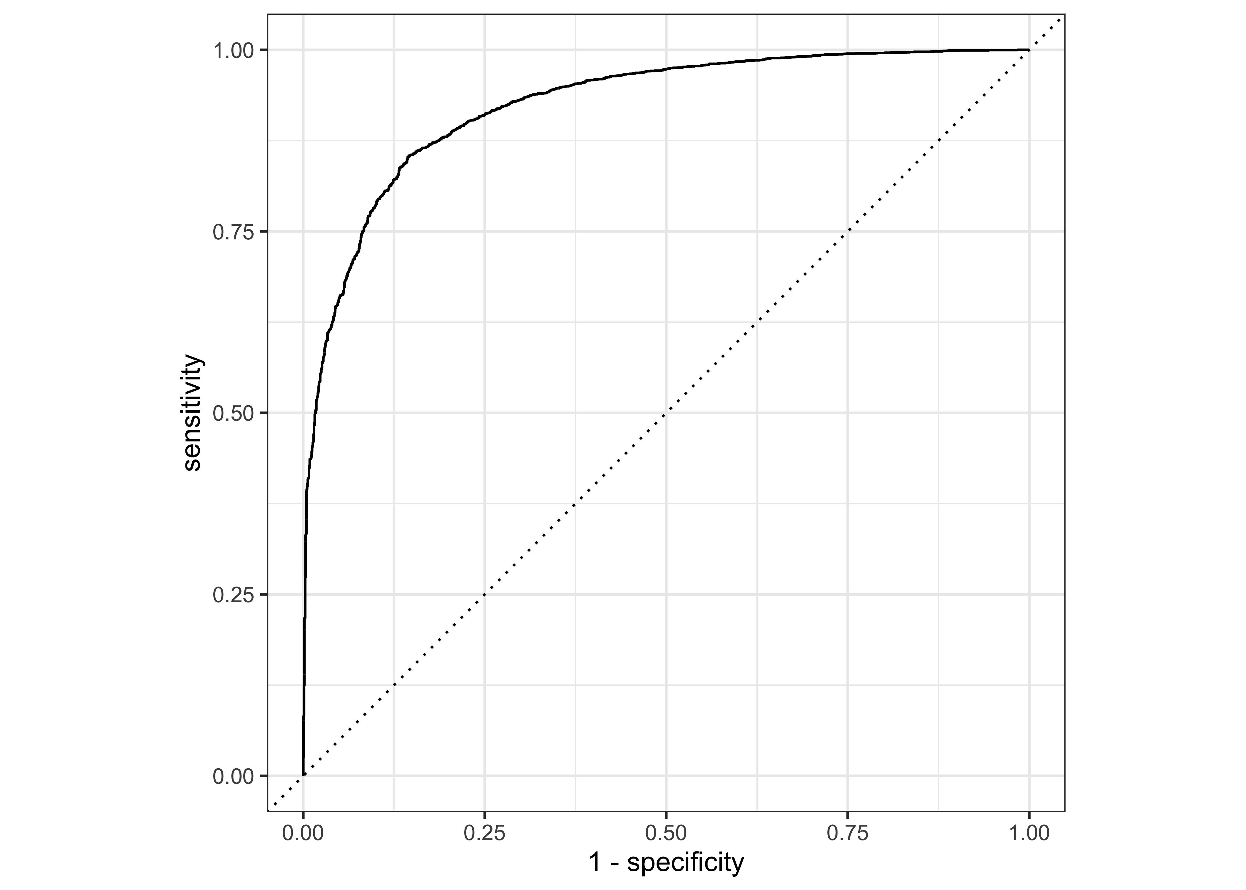
Based on all of the results, the validation set and test set performance statistics are very close, so we would have pretty high confidence that our random forest model with the selected hyperparameters would perform well when predicting new data.
